
1. Concrete Cast-in-place Column Cyclic Test
This is a simple example of a single cast-in-place (CIP) concrete column subjected to lateral cyclic loading. This test was performed and published by Dr. M.J. Ameli at the University of Utah. Dr. Ameli’s Ph.D. dissertation (Ameli 2016) is available for download for your reference. We will model this column with different element types available to understand the effect of modeling parameters. Before jumping into modeling, it is very important to decide the location of nodes. Since OpenSees does not have any graphical user interface (GUI), it is recommended to do a little brainstorming in deciding the node locations before starting any modeling. I generally draw the expected OpenSees model on a paper and follow it.
The column’s total height is 8.5 ft but the lateral loading is applied at a height of 8 ft in order to accommodate the actuator. If, in OpenSees model, we apply lateral loading at the total height of the column, we will not match the drift ratios recorded in the test. Therefore, we will put a node at the loading height.
The column’s total height is 8.5 ft but the lateral loading is applied at a height of 8 ft in order to accommodate the actuator. If, in OpenSees model, we apply lateral loading at the total height of the column, we will not match the drift ratios recorded in the test. Therefore, we will put a node at the loading height.
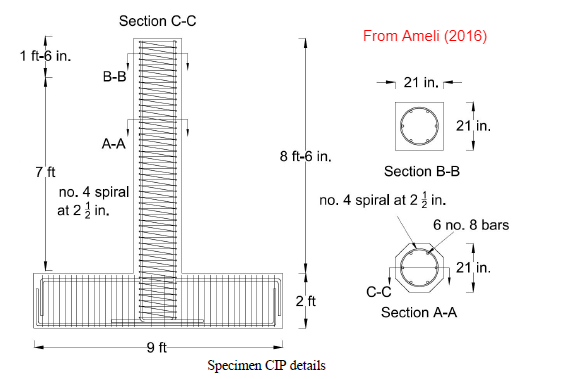
Disclaimer: The two drawings presented above are owned by Dr. M.J. Ameli.
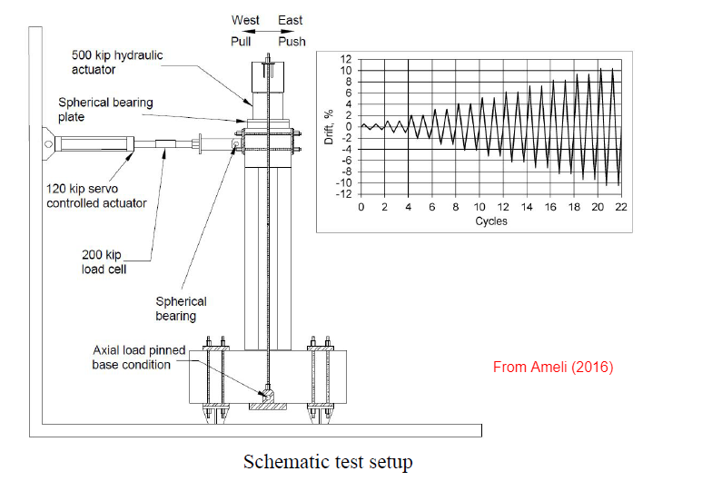
A vertical axial load was also applied to the column during Dr. Ameli’s test to simulate deck load. This load would generate P-delta effects in the column when pushed to higher lateral drift ratios. This vertical load was applied at the top of the column and not at the point of lateral loading. However, for simplification, we can apply vertical load at the point of lateral loading.
One of the nodes will be at the column bottom, which is the column-to-footing joint. Since during the test the footing was kept rigidly fixed by anchors, we don’t have to model the footing height. This simplification is not true for every situation. We have to be wise about the simplifications and assumptions.
It may seem useless to “brainstorm” since we only have two nodes in this model. But this process is useful for larger and more complex problems.
Now we can start our model. The first thing we have to do is to define our model space in OpenSees. For this example, a 2-dimensional model is sufficient. To initiate a 2-dimensional model with 3-degrees-of-freedom, use the following command,
Model BasicBuilder -ndm 2 -ndf 3
Then, we go on to define basic and dependent units. These units will later be used to set specimen dimensions and material properties. Any dimensions or values defined in dependent units will be converted to the basic units to perform calculations. For example, the column length defined as 10 feet will be converted to 120 inches.
The output of the program will also be reported in basic units.
The output of the program will also be reported in basic units.
Basic Units
set kip 1.0; # Kips
set in 1.0; # inch
set sec 1.0; # second
Dependent Units
set ft [expr $in*12]; # relate foot to inch
set lb [expr $kip/1000]; # relate pounds to kip
set ksi [expr $kip/pow($in,2)];
set psi [expr $lb/pow($in,2)];
set ksi_psi [expr $ksi/$psi];
set sq_in [expr $in*$in];
Universal Constants
set g [expr 386.2*$in/pow($sec,2)];
set pi [expr acos(-1.0)];
Once the units are defined, we will proceed to set column/specimen dimensions.
Dimensions
set Lcol [expr 8.00*$ft]; # Length of the column (distance between the base and the loading point)
set Dcol [expr 21.00*$in]; # Column Diameter
set Dbar [expr 1.00*$in]; # Diameter of each longitudinal rebar
set Abar [expr 0.79*$in*$in]; # Area of each longitudinal rebar
set s_bar [expr 2.50*$in]; # spacing between horizontal reinforcement / Spiral reinforcement
set cover [expr 2.00*$in]; # Concrete clear cover
Cross-Section Properties
set Acol [expr (($pi*$Dcol**2)/4)]; # Area of column
set Jcol [expr ($pi*($Dcol/2)**4)/2]; # Torsional Moment of Inertia
set I3col [expr ($pi*($Dcol/2)**4)/4]; # Moment of Inertia about minor axis
set I2col [expr ($pi*($Dcol/2)**4)/4]; # Moment of Inertia about major axis
Next, we will define material properties. Various material models are available in OpenSees for concrete and steel. Selection of material model can lead to convergence issues. For this example, we will use ‘Concrete02’ material model for concrete and ‘ReinforcingSteel’ material model for rebar. 'Concrete02' material model follows Mender's equation and hence needs f'cc (peak confined compression strength), ɛcc (strain at peak confined compression strength, f'cu (crushing strength of confined concrete) and ɛcu (crushing strain) to define the material. For 'ReinforcingSteel' material model, Fy (yield stress), Fu (peak stress) and E (modulus of elasticity). More information on the material property definition can be found on OpenSees command manual webpage.
Since our aim is to match the test performance of the column, we will use 'test day' strength parameters and not '28 day' strength parameters. All these parameters are provided in Dr. Ameli's dissertation. It is a good practice to define separate material properties for core and cover concrete to capture the true behavior of the section. However, for this example, we will just core concrete properties for the entire column section.
OpenSees uses numeric material tags for each material definition which is then applied to section definitions.
Now that we have defined the materials, column fiber section can be defined. In order to capture material non-linearity, fiber section will be used. In OpenSees, a numeric tag is associated with each section defined. This numeric tag is later used to assign the section to an element.
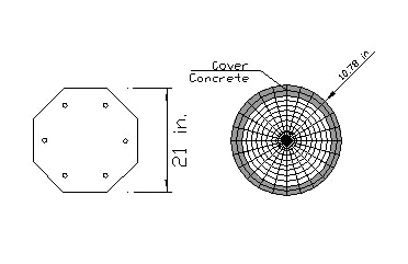
For simplicity, the octagonal column section can be modeled as a circular section with equal cross-sectional area. The diameter of the equivalent circular section is then used as "Dcol" which has been defined along with other dimensions at the beginning of the model script. The column cross-section is divided in to multiple non-linear fibers with appropriate concrete and steel properties. OpenSees command for Circular Fiber Patch is used to generate multiple concrete fibers over the column section.
For simplicity, the octagonal column section can be modeled as a circular section with equal cross-sectional area. The diameter of the equivalent circular section is then used as "Dcol" which has been defined along with other dimensions at the beginning of the model script. The column cross-section is divided in to multiple non-linear fibers with appropriate concrete and steel properties. OpenSees command for Circular Fiber Patch is used to generate multiple concrete fibers over the column section.
We have now successfully defined the required material properties and the section property for the column model. Let's start defining nodes and element. As discussed previously, we just need two nodes for this model. One node at the base and the other node at the loading height of the column. We will assume that the base node is fixed.
Since our model space is 2-dimensional, we need X and Y coordinates of each node. Also, the base node needs to be fixed in all degrees-of-freedom hence we will assign "1" for all three dofs.
Since our model space is 2-dimensional, we need X and Y coordinates of each node. Also, the base node needs to be fixed in all degrees-of-freedom hence we will assign "1" for all three dofs.
Before defining elements, we should define a 'Geometric Transformation'. This establishes a relationship between the global coordinate system and the local coordinate system of the elements. For a 2-dimensional space, this relationship is simple and straight forward. Therefore the only thing in this model we need to choose if we want PDelta effect or not. Since, this is a non-linear analysis with a significant axial load on the column and large lateral displacements, we should include PDelta effects.
A numeric tag is assigned to each geometric transformation definition which is later used while defining element connectivity. (I generally define a "Transformation Type" separately, as you can see below, to make it easier for me to understand code for large/complex models. I define different transformation types for beams, columns in different locations. Thus I can just change the "TransfType" parameter to "Linear" or "PDelta" without getting confused each time.
While defining the elements, we need to assign number of integration points along the length of the element. For a non-linear element, the predefined fiber-section is assigned to each integration point. A minimum of 2 integration points can be assigned for a linear moment distribution along the element length. However there is no upper limit, it is recommended to assign 5 integration points to capture non-linear distribution of the moment along the length. For this example, we will start with 2 integration points. This will only calculate the nonlinear behavior at the bottom and the top of the column element.
* Later we will compare the effect of number of integration points on the output.
Since we are trying to perform a static displacement controlled analysis, there is no need to assign mass to the nodes. Pushover and cyclic analysis can be performed without any mass assignment. This is possible because OpenSees does not convert mass to weight for gravity loads internally. We can assign loads in vertically downward direction as "weight". However, to calculate mode shapes, modal periods and dynamic analysis, we need to assign mass.
To follow the test setup, first we will define the axial load applied on the column. This axial load is a representative of the superstructure weight. Hence, we can define a quantity "Weight" and then convert it into "mass". This mass will be assigned in all the translational degrees-of-freedom. A "-Weight" load will be assigned in 2nd degree-of-freedom which is global Y direction.
All the loads are assigned under a load pattern command. For static load, a linear load pattern is suitable.
The model definition is now complete. We will now analyze the structure for gravity loads. It is important to check if the structure is stable for gravity loads before performing any lateral analysis.
Before performing the analysis, we should define appropriate recorders. "file mkdir Gravity" is a Tcl command to create a folder named "Gravity". All the recorders will save the output in this folder. The first recorder is for lateral reaction at node 1, i.e. base of the column in 2nd degree-of-freedom. Second recorder is to record stress and strain for concrete fiber at column center.
Before performing the analysis, we should define appropriate recorders. "file mkdir Gravity" is a Tcl command to create a folder named "Gravity". All the recorders will save the output in this folder. The first recorder is for lateral reaction at node 1, i.e. base of the column in 2nd degree-of-freedom. Second recorder is to record stress and strain for concrete fiber at column center.
Static analysis is performed as follows. Most of the models will converge for gravity analysis using the following lines of code. For complex models, if convergence issues arise, you can experiment with a different "system", "test" and "algorithm" types.
Now we can perform static pushover analysis. Pushover analysis is a static displacement controlled analysis. "ControlNode" is assigned a lateral displacement in lateral direction ( 1 dof in this example) up to a maximum displacement of "Dmax". To avoid convergence issues, the analysis should be performed in small steps "Dincr". The analysis will have "Dmax/Dincr" total number of steps.
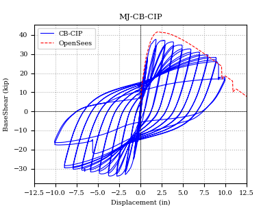
The analysis will converge and the output files will be saved in a folder named "Pushover". Base shear vs lateral drift can be plotted along with the test data to see how well our model predicts the test output. It is obvious that the numerical output does not match the test data very well. You can tweak some material parameters to match the behavior.
Next, you should try to perform a cyclic analysis to see how the cyclic behavior of the numerical model matches with the test.
References:
1) Ameli M. J., 2016. "Seismic Evaluation of Grouted Splice Sleeve Connections for Bridge Piers in Accelerated Bridge Construction". Ph.D. Dissertation, University of Utah.
2) OpenSees (http://opensees.berkeley.edu/)