
NOTE:
1) This rendering works only for 3D stick-beam models I.e. models involving beam-column elements and link elements only. It will not work for shell or 3D solid elements.
2) The vertical axis of the model should be in the global Z-direction. If otherwise, you will have to make minor changes in the plotting script.
You can download the Tcl and Python scripts used in this tutorial by clicking the link above or from my GitHub page..
Get_Rendering.tcl : Call this file from the main model file by writing source Get_Rendering.tcl AFTER performing the Eigen analysis.
StructurePlot.py : Visualizes the 3D model using Python's basic Matplotlib library.
StructurePlotMayavi.py : Visualizes the 3D model using Mayavi.
StructurePlotly.py : Visualizes the 3D model using Plotly.
PlotModeShape.py : Visualizes any recorded modeshape of 3D model using Python's basic Matplotlib library.
OpenSees is an awesome platform for structural analysis which gives the users freedom and flexibility of running analysis on any machine including cloud. One of the challenges many users face is in visualizing complex structures. I use Python to visualize complex structures and plot mode shapes. Python, unlike Matlab, is open-source just like OpenSees and can utilize various plotting/visualization libraries such as Matplotlib, Mayavi, Plotly, Paraview, etc.
There are two steps involved in visualizing an OpenSees model,
1) record coordinates of all the nodes, elements and their connecting nodes in OpenSees,
2) put the recorded data in a 3D plot using Python.
To record node coordinates and elements, there is no need to run an analysis. Just source the OpenSees model file to complete the model definition. To record mode shapes, you will have to run an Eigen analysis. Therefore, rendering the shape of the model can be helpful in visualizing any wrong or missing connections in the model.Once the OpenSees model is running successfully for gravity and modal analysis, you can start recording mode shapes.
Recording Node Coordinates
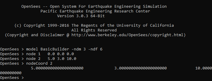
The OpenSees command nodeCoord $nodeTag spits out the coordinates of the node $nodeTag. For example, the coordinates of node 2 in an OpenSees model can be obtained by typing the command nodeCoord 2 (see the image below). For a model defined in 2D space (-ndm 2 –ndf 3), this command will give X and Y coordinates.
There are two steps involved in visualizing an OpenSees model,
1) record coordinates of all the nodes, elements and their connecting nodes in OpenSees,
2) put the recorded data in a 3D plot using Python.
To record node coordinates and elements, there is no need to run an analysis. Just source the OpenSees model file to complete the model definition. To record mode shapes, you will have to run an Eigen analysis. Therefore, rendering the shape of the model can be helpful in visualizing any wrong or missing connections in the model.Once the OpenSees model is running successfully for gravity and modal analysis, you can start recording mode shapes.
Recording Node Coordinates
The OpenSees command nodeCoord $nodeTag spits out the coordinates of the node $nodeTag. For example, the coordinates of node 2 in an OpenSees model can be obtained by typing the command nodeCoord 2 (see the image below). For a model defined in 2D space (-ndm 2 –ndf 3), this command will give X and Y coordinates.
Since we want coordinates of all the nodes in the model, we need to create a text file in which we can write coordinates of the nodes, get a list of all the nodes defined in the model and write coordinates of all the nodes in the generated list using the nodeCoord command in a Tcl loop.
To create a text file, first, assign the name of the file to a variable and then open the file with read+write+append permission (w+).
Quick Information on Tcl file operations:
r : opens files for reading only
w : opens files for writing but deletes existing text before writing
w+ : opens files for writing by appending the text, i.e. does not delete the existing text.
Now, get a list (named listNodes) of all the nodes defined in the OpenSees model using getNodeTags command. This list contains node tags in ascending order.
Now, we create a Tcl loop to write tag and coordinates of each node in the listNodes to the output file RecordNodes.out created previously. Foreach loop in Tcl is a good option to loop over the list since the length of the list will be different in each model. The coordinates of each node in the list are set to a temporary list (tempNode) which is then written to the output file (fieldNodes) along with the tag of that particular node. This temporary list is then unset and is ready to be assigned new values in the next iteration.
The following image shows how the RecordNodes.out file will look like for a model defined in 3D space, with node numbers (tag) in the first column and corresponding coordinates in remaining columns.
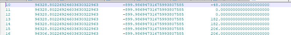
A view of file "RecordNodes.out"
Recording Elements
A similar procedure is followed to record the elements and their connecting nodes in a file. First, create an output file RecordElements.out and open it with write+append permission,
Get a list of all the elements defined in the model,
Nodes connected by an element with tag eleTag in OpenSees can be obtained by using the command eleNodes $eleTag. Loop over the element list to write the tag and nodes connected by each element to the output file,
The RecordElements.out file will look like the following image for a model defined in 3D space, showing element number (tag) and corresponding connected nodes (a total of 3 columns).
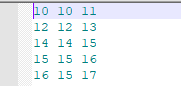
A view of the file "RecordElements.out"
Recording Mode Shapes
Modal displacement of any node can be recorded using node recorder in OpenSees with the help of the following command,
recorder Node -file FileName.out -nodeRange 1 2 -dof 1 2 3 "eigen 1"
The above command will record displacement of nodes 1 and 2 in the first three degrees-of-freedom (I.e. 1, 2, 3) for mode shape 1 (eigen 1) in an output file named FileName.out.
Now we want to record modal displacements of all the nodes in the model in order to plot the mode shapes. Since the node list we created earlier (listNodes) recorded the nodes in ascending order of their numbers (tags), we need the first and the last number of the list to assign a node range.
Total number of the nodes in the list (N) or the length of the list can be obtained as,
set N [llength $listNodes]
here the first node in the list : [lindex $listNodes 0]
and the last node in the list : [lindex $listNodes [expr $N-1]]
I would recommend creating a separate folder to save the data for the mode shapes. Here we will create a folder called ModeShapes and each mode shape data will be saved in a separate output file. For a model in 3D space, we have to record displacement in three translational degrees-of-freedom. For a 2D model, only –dof 1 2 are needed.
Finally ... Plotting Time
It is very helpful to visualize the mode shapes in a 3D interactive plot. A plot you can zoom-in, rotate and change perspectives for a better presentation. Here I will use Python’s most basic plotting library Matplotlib, a separate scientific visualization library Mayavi, and an awesome web-based platform Plotly to visualize our model.
Using Matplotlib
Assuming that you have already setup Python, Numpy, and Matplotlib. Now import the necessary libraries,
Now, initiate a 3D plot space.
Read the node coordinates from the file RecordNodes.out,
Define a Python function nodecoords to get coordinates of any node with a tag nodetag. This function is then called in a loop to read and plot each element one by one.
Create a loop to read elements from the file RecordElements.out and plot each element in the 3D figure defined previously.
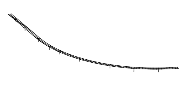
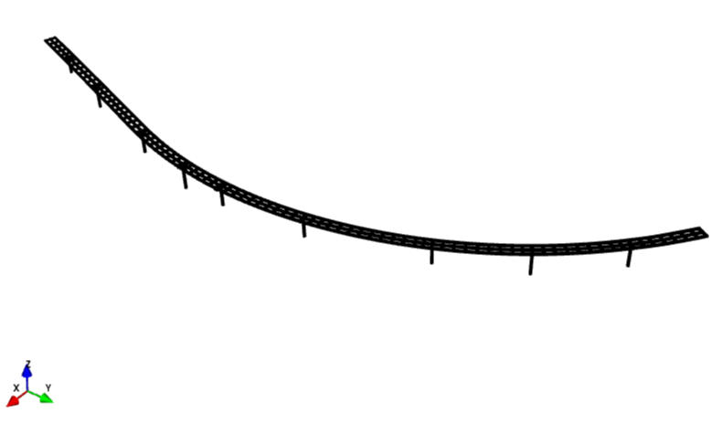
A multi-span bridge rendered with Python and Matplotlib.
Matplotlib library was created to plot figures and not primarily to interact with the data. Therefore, it is sluggish when it comes to interacting with a large number of data-set. For example, if you want to change the view angle of a big OpenSees model, it takes time to refresh the plot. Mayavi, on the other hand, is amazingly fast in changing view angles and perspectives. This is important while realizing the mode shapes of a large model.
Using Mayavi
Mayavi is a great tool for scientific visualization of 3D data. It provides a clear user interface to interact with data using Python (similar to Matplotlib). Mayavi utilizes widely used VTK (Visualization ToolKit) in the background through Python-based library.
Import Mayavi library into Python environment and define an empty 3D plot space.
Now the best part is that everything remains the same as the previous script (Matplotlib) except the plot function. Here we will plot using mlab instead of ax.plot,
You can experiment with the tube_radius which governs the thickness of the plotted elements. The following image shows the output of Mayavi.
A multi-span bridge rendered with Python and Mayavi.
Model View Using Plotly
Sometimes sharing the model and mode shapes with your teammates is required. Wouldn’t that be awesome if they could interact with your model without going through the hassle of installing Python or Mayavi or learning these tools? Here Plotly is your friend. Plotly is a .html based opensource plotting library that can convert your 2D and 3D plots into interactive web-based plots. Plotly plots can be generated offline (running on a local machine) and online (if you want to embed the plots on a website).
The offline interactive plots can be saved as .html files on your machine and can be shared via email. On double-clicking, they open in your local browser as interactive plots (models or mode shapes in our case). Opening a .html file/plot does not require Python or Plotly installed. Click here to download an offline model render of the same bridge to use on your local machine.
Plotly offers a free/community account where you can store up to 100 online plots/figures to share with the world. These can be easily embedded in a website or web-based reports. There is no need to send the plot files separately.
Once you have successfully installed Plotly, import it into the Python environment,
Plotly go is used to plot the data and Plotly.io is needed for input-output operations (such as saving plots as .html). The plotting loops created will remain the same as the previous two methods. There is a specific way to parse data and style in Plotly.
Create an empty figure space and define a function nodecoord as described earlier,
Plot each element is a loop (follow Plotly tutorial for specific commands and style),
Finally, save the figure as a .html file in the same folder using Plotly.io function. If you want the plotted figure to open in your web browser automatically, set auto_open=True.
Here is an interactive OpenSees model render hosted on Plotly account. Go ahead and rotate the model by click, hold and move the cursor.
